Image Warping and Mosaicing
Homographies
To warp images, we must first create the homography matrix, H, by recovering 8 unknown entries of the 3x3 matrix. We can find the 8 unknowns, h, by having 4 points to sample from the source image and 4 corresponding points from the warped image. These 4 sets of points are plugged into a matrix A and a set of points, b, to use least-squares to get h. Then having h, we can form H.
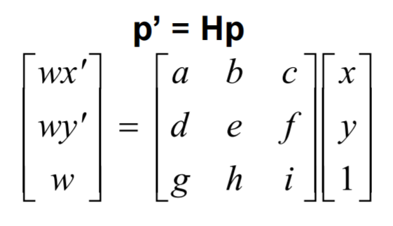
Homography Matrix
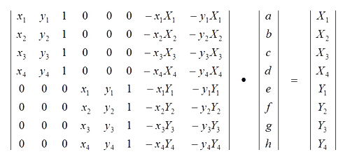
Ah = b
Warp the Images
To warp the image into a desired warp we do the following:
- Given 4 or more correspondences, calculate the homography matrix, H.
- Use the corners of the original image to create the bounding box of the warped image by passing the corners through H.
- Then use inverse warping to create the warped image
Image Rectification
All the following are pictures with planar surfaces warped so the plane is front-parallel.
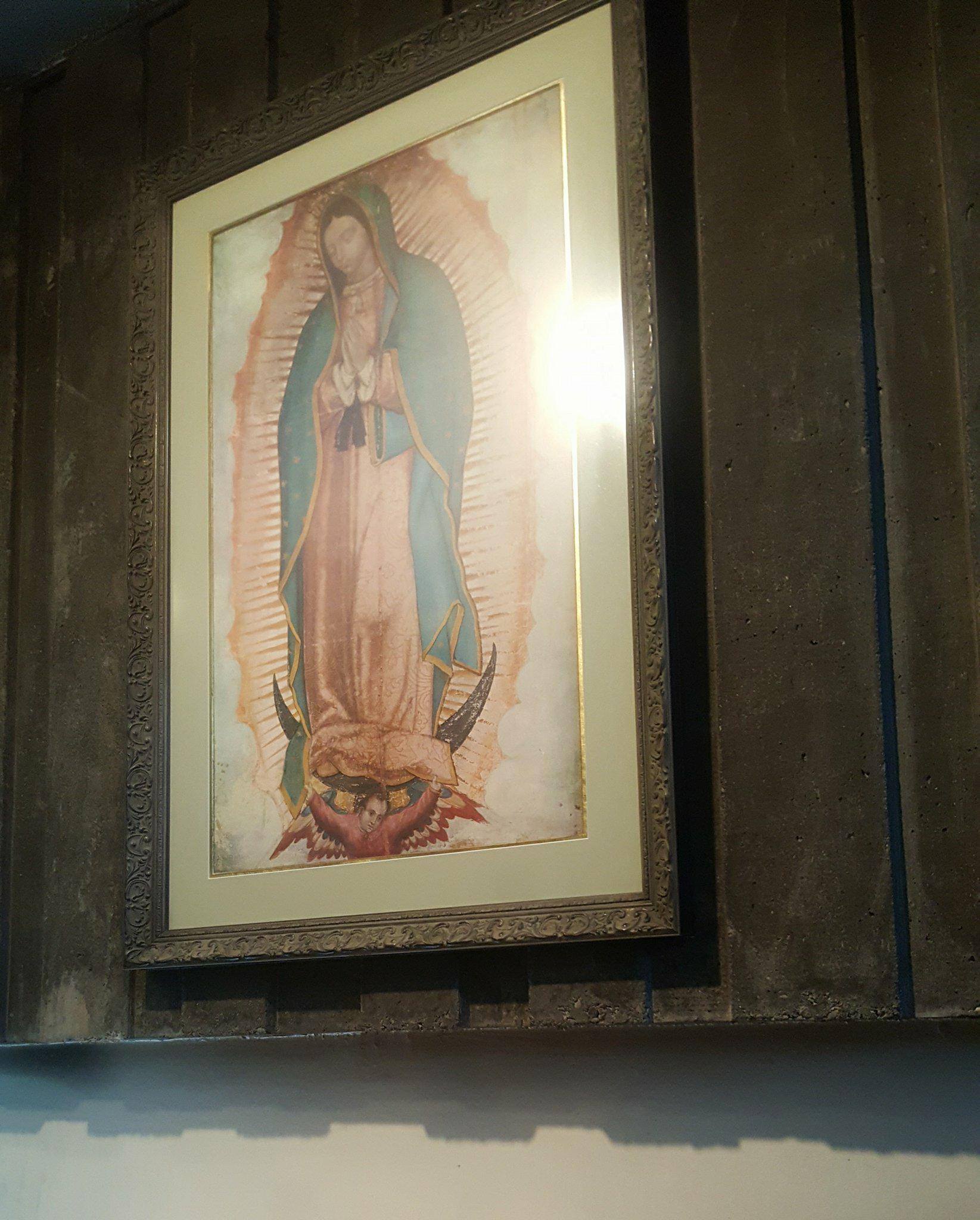
Our Lady of Guadalupe
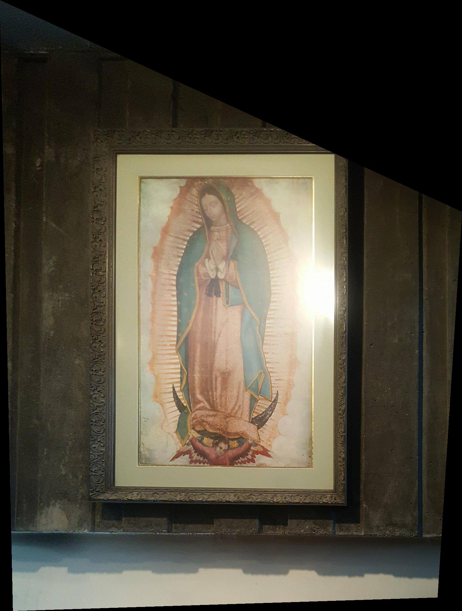
Warped Guadalupe

SF Japanese Tea Garden

Warped Tea Garden
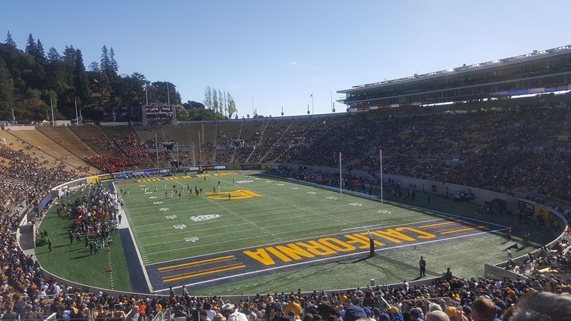
Memorial Stadium
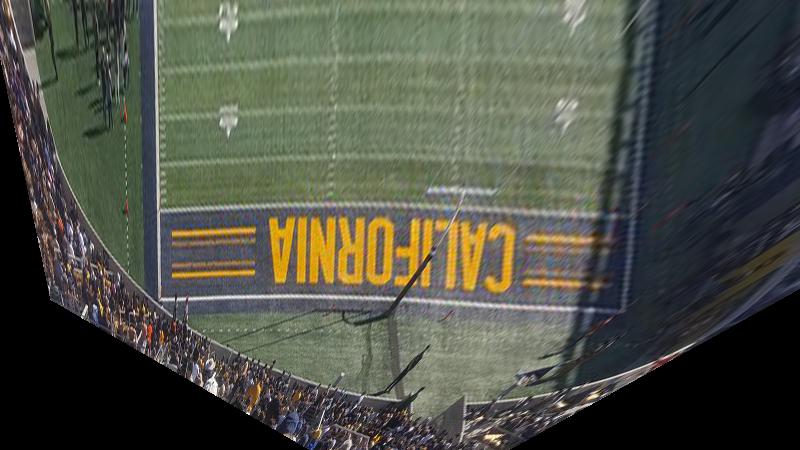
California
Blend the images into a mosaic
For the next part, I combined 2 similar images to create a mosaic panorama. We accomplished this by doing the following:
- Plot points on both images where the same objects would correspond to the same points on both images.
- calculate the homography matrix, H.
- Warp one of the images to match the projection of objects of the other images and shift both images accordingly to fit into a frame and overlap.
- Blend (I used both weights and multiresolution blending)
The following are results as I used Yosemite as a clear example of plotting points, warping and overlaying, then blending:
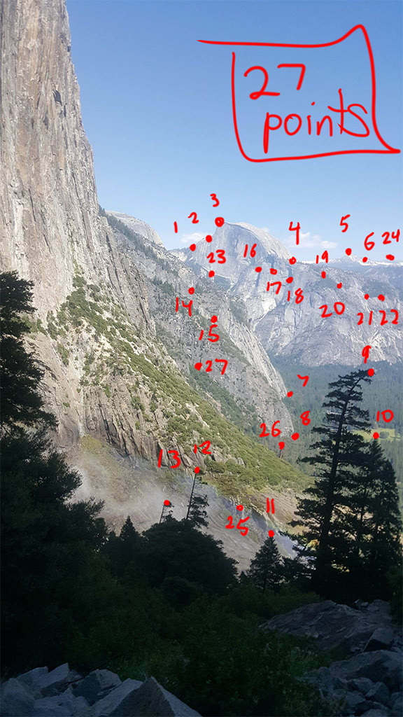
Yosemite points

Lake Tahoe points
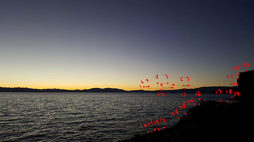
More Lake Tahoe points
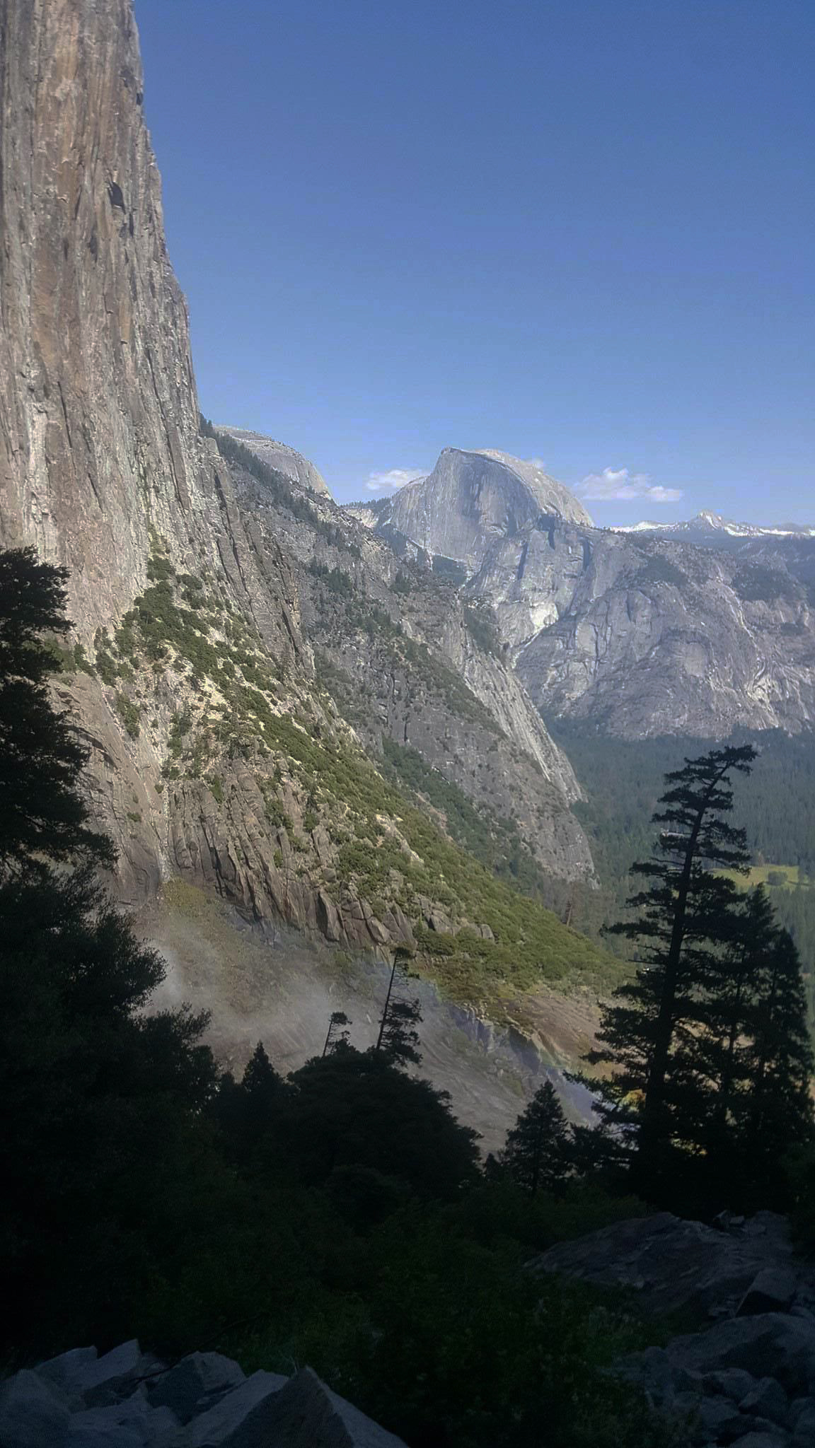
Yosemite Left
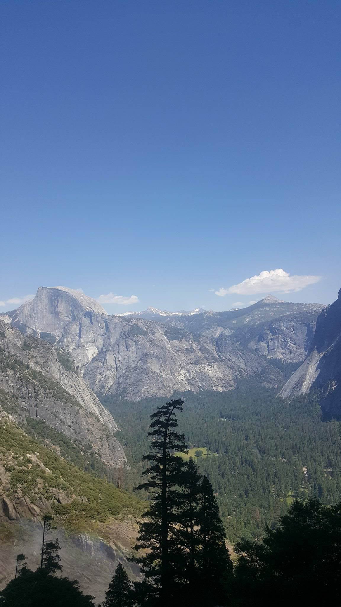
Yosemite Right

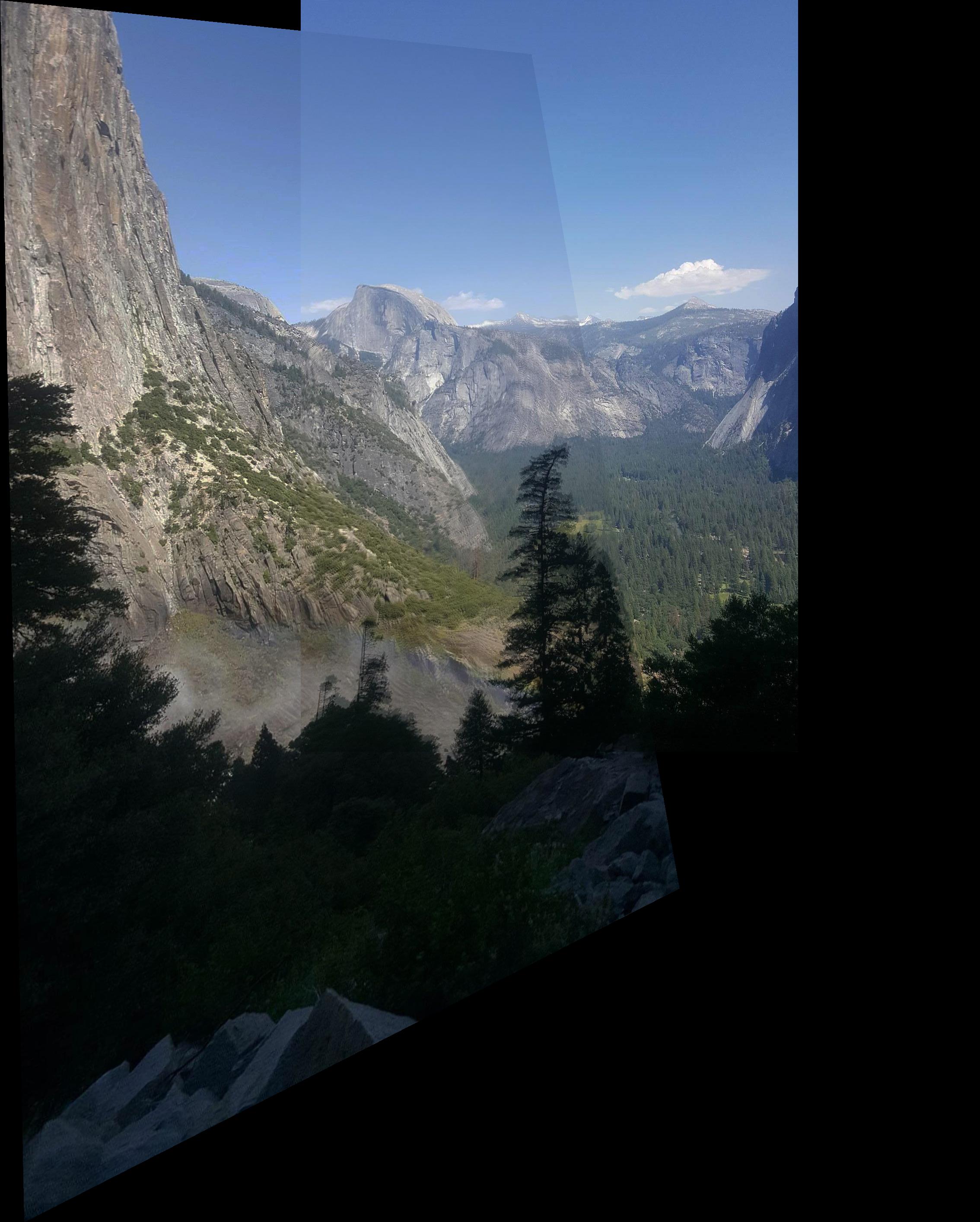
Half Dome overlay
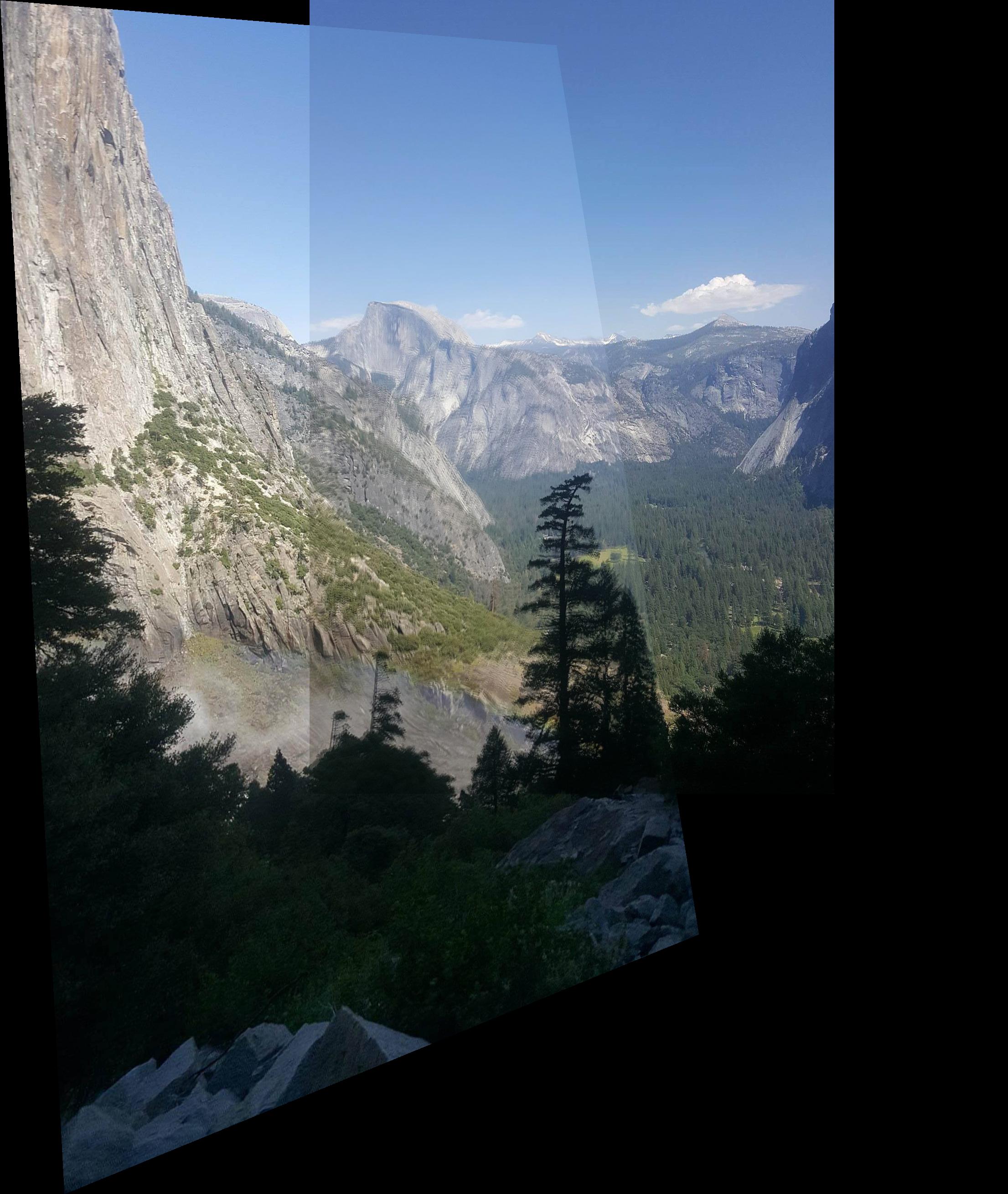
Half Dome weights
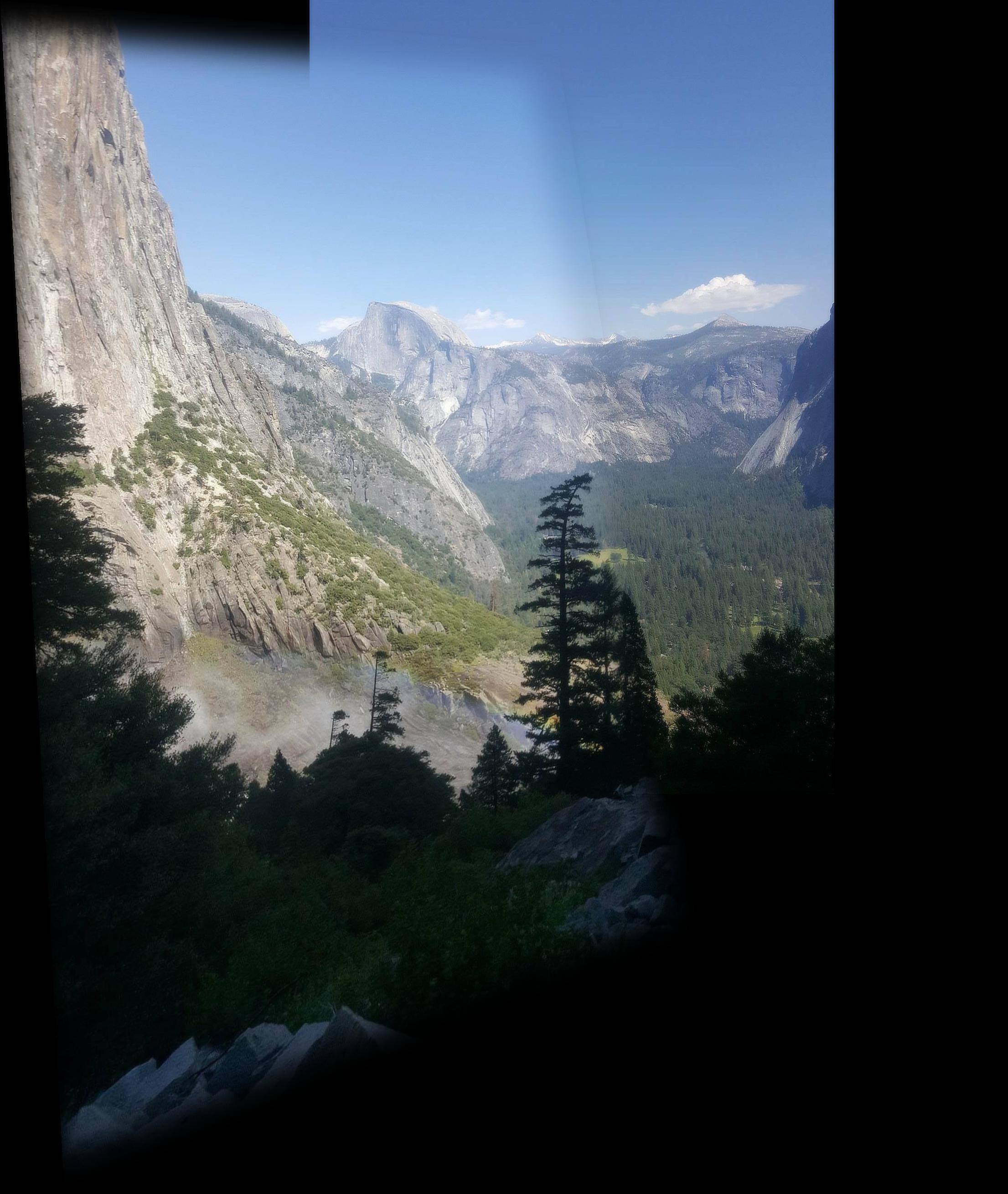
Half Dome multiresolution blending
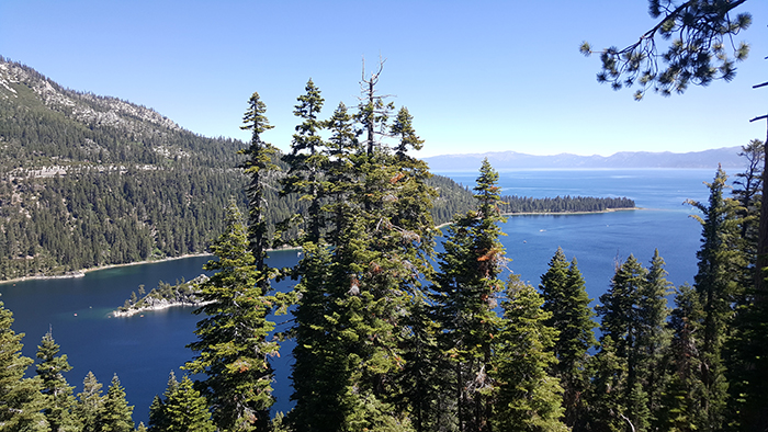
Lake Tahoe Left
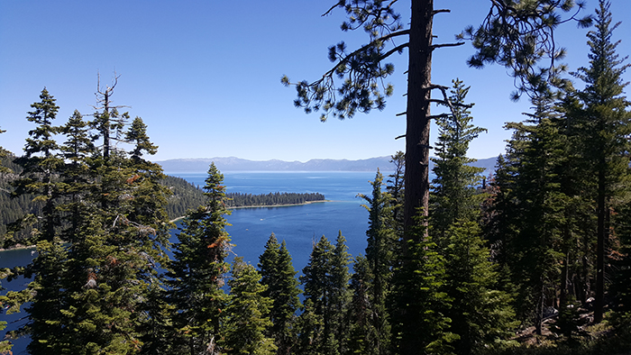
Lake Tahoe Right
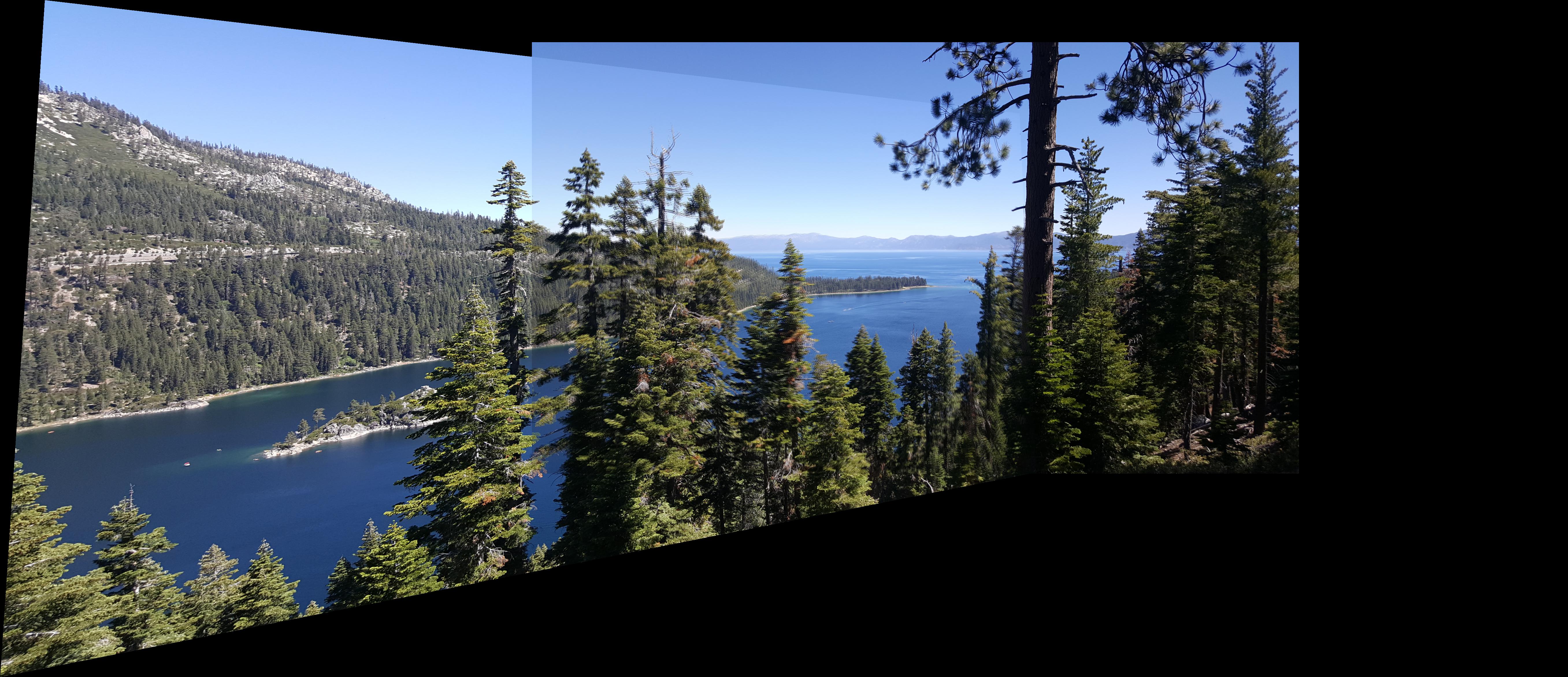
Lake Tahoe weights
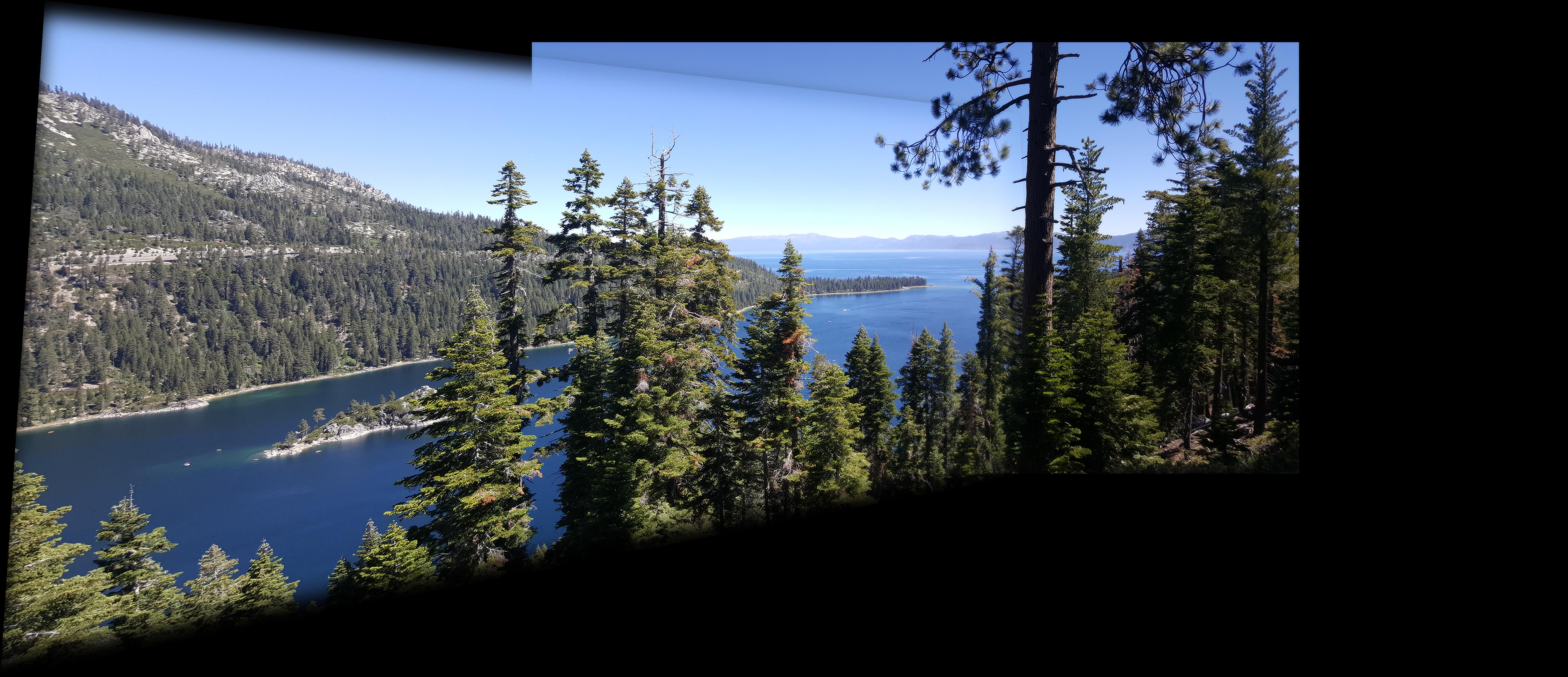
Lake Tahoe multiresolution blending

More Lake Tahoe Left

More Lake Tahoe Right
More Lake Tahoe weights

More Lake Tahoe multiresolution blending
Adaptive Non-Maximal Suppression
By getting the Harris Corners as given to us, we have to many points that are too close to each other. Using Adaptive Non-Maximal Suppression, we can lower the amount of points and space the chosen Harris Corners. We do this by getting the minimum r_i for each corner where r_i = min|xi-xj| for all j such that f(xi) < 0.9f(xj). f in this case is the corner intensity. We then take the points based on r_i such that we find all the points greater than or equal to r_i where the number of points greater than or equal to r_i is 500. We then use thoe 500 well spaced points, p, moving forward
Feature Descriptor
Now we have to get descriptors of each point. We take 40x40 patches for each point and create 8x8 normalized patches that is flattened into a 64 dimensional vector that can be used for feature matching between 2 images.
Feature Matching
For each descriptor in the first image, we pair it with a descriptor from the second image if the ratio of the closest matching descriptor to the second closest descriptor of the second image is less that 0.4.
RANSAC
Lastly, we create a homography matrix by running 15000 iterations of picking 4 random points, getting the homography matrix, and picking the homography that includes the most inliers using points from feature matching. Then we use the inliers of the homography matrix to form a least squares homography matrix.
The following image has yellow points to represent the results of Adaptive Non-Maximal Suppression, the blue points represent the results of Feature Matching, and the red points represent the results of the points used in RANSAC.
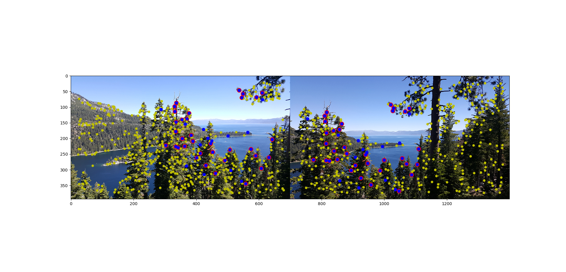
Points as results of RANSAC
The following is the manual points compared to RANSAC points:
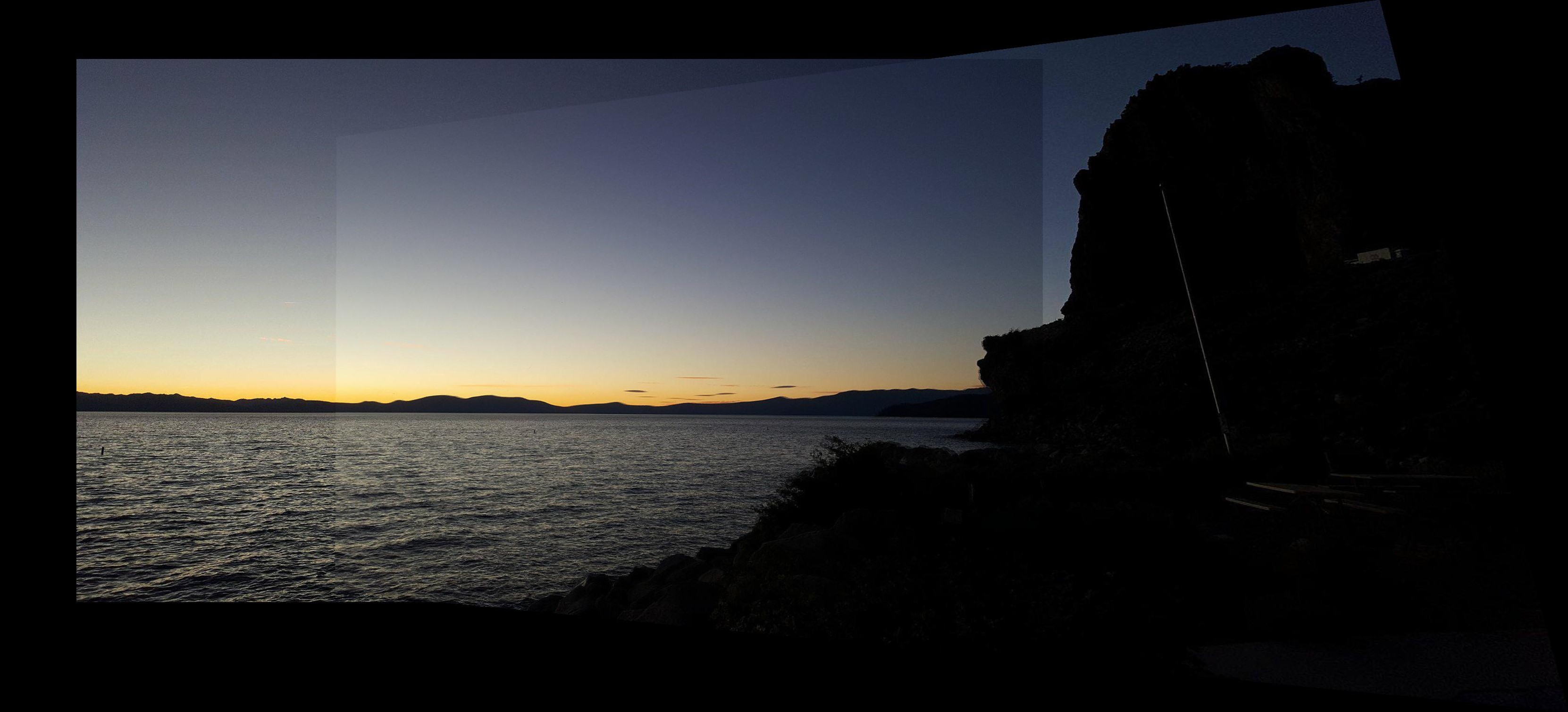
Tahoe Sunset Manual weights
Tahoe Sunset RANSAC weights
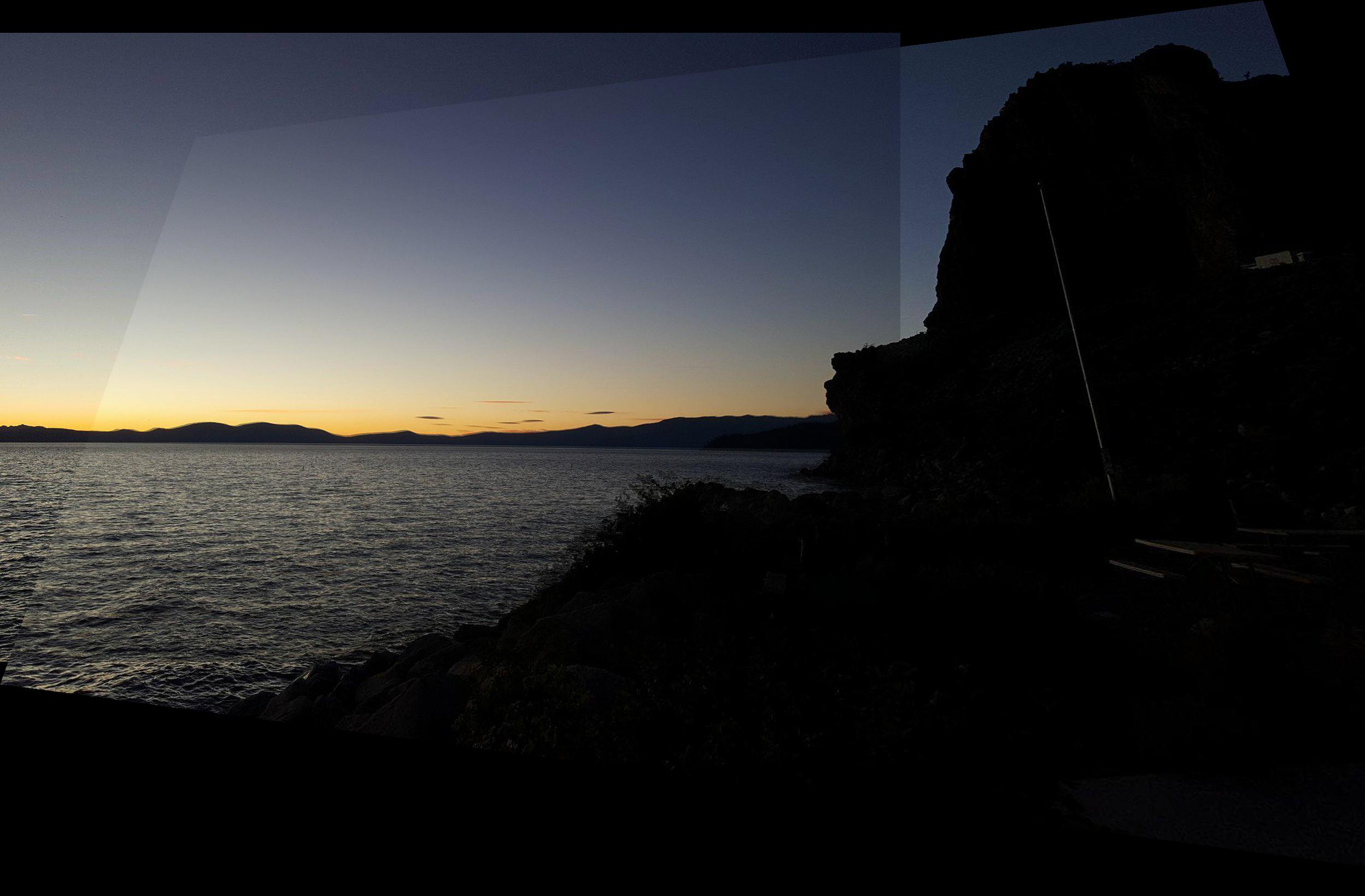
Lake Tahoe Manual weights

Lake Tahoe RANSAC weights
Half Dome Manual weights
Half Dome RANSAC weights