PathTracer
The goal of this project is to create a path tracer that produces images from meshes that are lit up through global(direct and indirect) illumination given a light source. Along with that, besides diffuse objects, glass and mirror objects could be rendered as well. However, to achieve this final result, rays first had to be created from the camera that point to the mesh. To calculate where the rays hit the mesh, BVH(Bounding Volume Hierarchy) algorithms were needed to be able to split a mesh into groups so a ray can easily find where an intersection takes place instead of searching through every primitive on a mesh. For each point where a ray's closest intersection occurs, the amount of light directly from a light source that reaches the point of intersection has to be calculated, direct illumination. Along with that, the amount of light that reaches a a point of intersection from other light rays not directly from a light source, but from extra light reflecting or refracting from other objects have to be calculated as well, indirect illumination. The sum of those two lights produce the final images. Some materials such as mirrors have special properties to reflect light and materials such as glass have special properties to reflect some light and refract other light rays. So these were materials and properties that were implemented as well.
Part 1: Ray Generation and Intersection
To generate light rays that find its ways to the pixels of the camera, we don't start from the light to find the rays that hit the camera because we would generate more rays that needed. So we start from the camera and create rays that would hit the light because radiance entering a pixel on the camera from a point, p, is equal to the radiance leaving that pixel towards the point p. So we generate a ray starting from a point from the camera using a function generate_ray() in camera.cpp. That ray takes in coordinates x and y where both coordinates range from 0 to 1. We use the (x, y) coordinate to find its coordinate on a 3D plane where the bottom left of the plane is (-tan(radians(hFov) * .5), -tan(radians(vFov) * .5), -1), and the top right of the plane is at ( tan(radians(hFov) * .5), tan(radians(vFov)*.5), -1). hFov is the horizontal field of view angle and vFov is the vertical Field of view angle given as camera parameters. We interpolated where the point (x ,y) is also on the plane where
x = -tan(radians(hFov) * .5) * (1 - x) + tan(radians(hFov)*.5) * x
y = -tan(radians(vFov) * .5) * (1 - y) + tan(radians(vFov)*.5) * y
        z = -1
The new vector is converted to world space then normalized, then a ray is generated with an origin at a camera parameter pos, a direction towards the new vector, a min_t is nClip and max_t is fClip where nClip and fClip are camera parameters. That means the ray vector goes from pos, towards, to the pixel on the camera. This new ray is returned.
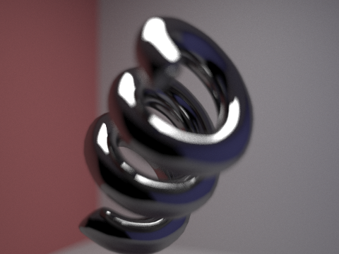
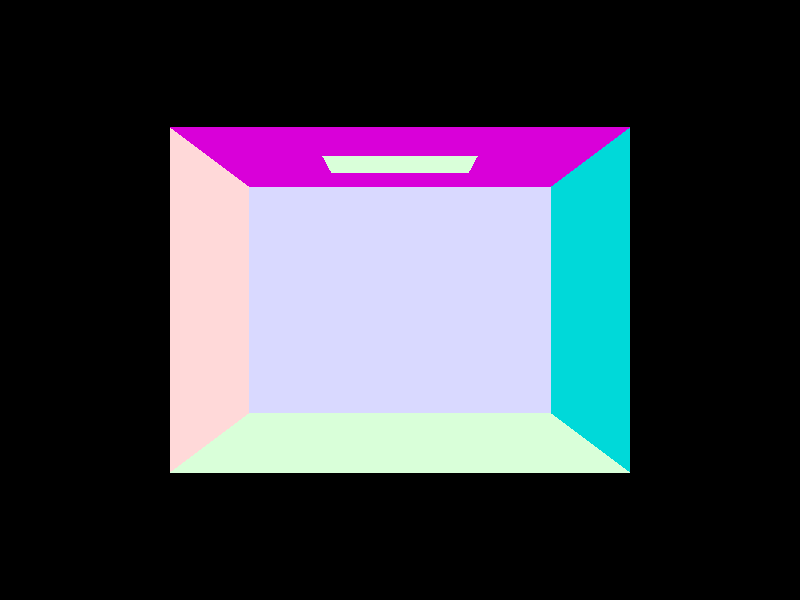
Next in the function raytrace_pixel() in pathtracer.cpp. given a 2D point, (x, y) within a plane with a width and height of a sampleBuffer, which is a pathtracer parameter. Depending on a pathtracer parameter, ns_aa, we generate ns_aa random rays that have a 2D coordinate between (x, y) and (x + 1, y + 1). If ns_aa is only 1, the ray generated is (x + .5, y + .5). For each ray we call a function trace_ray() which takes in a ray, our generated rays, and a boolean which is marked as true since it is a ray from the camera and returns the radiance that reaches a camera pixel from each generated ray, add the radiance from each ray, then average by dividing by ns_aa. This averaged radiance is returned and displayed in Figure 1 to Figure 4.
Lastly, since all the scenes are made of primitives, triangles and spheres, intersect functions for triangles and spheres were tested to see if a ray hits a primitive. To see if a ray hits a triangle, the Möller-Trumbore algorithm was used. Given the ray, r, and the 3 points of a triangle, p1, p2, and p3. We calculated some vectors
e1 = p2 - p1
e2 = p3 - p1
s = r.origin - p1;
s1 = r.direction x e2
s2 = s x e1
First a time, t, was calculated to see if t lies between the r's min_t and max_t. If it doesnt, then the hit is not a true hit, the function returns false.
t = dot(s2, e2) / dot(s1, e1);
Then using the calculations above the barycentric coordinates, of the ray compared to the points of the triangle, (b1, b2, b3), can be calculated.
b1 = dot(s1, s) / dot(s1, e1);
b2 = dot(s2, r.direction) / dot(s1, e1);
First b1 is calculated and if b1 is less than zero or greater than 1, the ray does not hit the triangle, returning false. b2 is then calculated and if b2 is less than 0, the ray also does not hit the triangle. In barycentric coordinates, b1 + b2, + b3 = 1, so if b1 + b2 is greater than 1 already, false is returned.
r.max_t = tr.max_t is updated to make sure nothing behind the triangle also cause a hit. If the intersect function also takes in a Intersection isect
isect->t = t;
isect->n = (1 - b1 - b2) * n1 + b1 * n2 + b2 * n3;
isect->primitive = this;
isect->bsdf = get_bsdf();
After that, true is returned. Figure 1 and Figure 2 show the results of completing everything talked about up to this point.

For sphere intersect that takes in a ray, r, the discriminant is calculated by first finding a, b, and c.
oMinusc = r.origin - sphere's center
a = dot(r.d, r.d)
b = dot(2 * oMinusc, r.d)
c = dot(oMinusc, oMinusc) - r2;
discriminant = b^2 - 4 * a * c
If the discriminant is less than 0, there is no intersection, false is returned because the ray doesn't intersect the sphere. Otherwise, t1 and t2 are calculated, the times of intersection.
t1 = (-b + sqrt(discriminant)) / (2 * a)
t2 = (-b - sqrt(discriminant)) / (2 * a)
If t1 is greater than t2, they are swap, then if t1 is less than zero, the ray is inside the sphere or doesn't hit the sphere, so t1 is set to equal t2. Then if t1 is still negative, that means the ray didn't hit the sphere at all so false is returned. Then there is a check to see if t1 and t2 intersect the r's min_t and max_t. If not, false is returned. Otherwise,
r.max_t = tJust like with triangle r.max_t is updated to make sure nothing behind the triangle also cause a hit and isect is updated if it is a parameter.
isect->t = t1;
isect->n = (r.o + i->t * r.d - o).unit();
isect->primitive = this primitive;
isect->bsdf = get_bsdf();
isect->n is set to the unit vector pointing from the origin towards the point of intersection, isect-primitive is the sphere we're checking if the ray, r, intersects it. And each each primitive has a material that get_bsdf() returns. (I noticed in Figure 3, my normal shading was weird because I forgot to turn isect->n into a unit vector.) The final result is in Figure 4 Afterwords, true is returned and the ray, r, and the sphere have a true intersection. All the Figures up to now contain only a few primitives. Besides the gem scene, Figure 2, which has about 200 primitives, the other scenes have less than 15 primitives each.
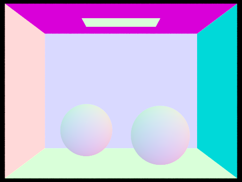
Figure 3: Spheres with bad normals.
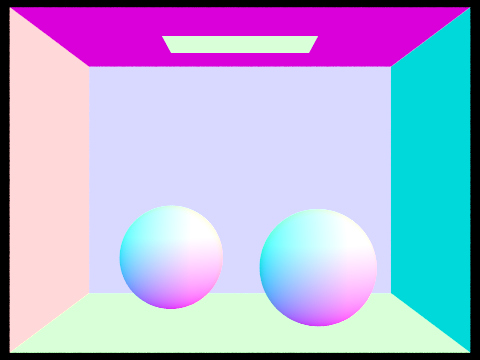
Figure 4: Fixed spheres in a Cornell box.
Part 2: Bounding Volume Hierarchy
Given a scene with many primitives, it is best to split the primitives into smaller sub groups so it'll make it easier to check the sections that a ray intersects in the scene rather than check each primitive in the scene and see if a ray hits. To do this a BVH construction algorithm, construct_bvh() in bvh.cpp, is used. The algorithm starts by creating a bounding box for all the primitives given as an input. A new node is created with the new bounding box then if the amount of primitives in the input is less than or equal to a given input of max_leaf_size, the new node's prims is equal to the input primitives and the node is returned. Otherwise, the node needs to be split into left and right nodes. The bounding box is 3D so the dimension of the largest size is the dimension that will be split. The midpoint of that dimension becomes the split point and every primitive given is put either to the group left of the split point and equal to the split point, or to the group right of the split point. If both the left and right both have primitives in them, the algorithm is recursively called onto nodes containing the left and right groups. On the other hand, if the left or the right group is empty, the next largest dimension is chosen to split the primitives. If that fails, last dimension splits the primitives. And if all 3 dimensions fail to split the primitives, the node's prims is then set equal to the input primitives. After the recursion of left and right nodes or failure to split, the node is returned.
After the sub groups are created, the groups can be used to check where and if a ray intersects a scene using a BVH intersection algorithm, intersect() in bvh.cpp. First, the algorithm checks if the ray intersects a node's bounding box using an intersect function in bbox.cpp. If the ray doesnt intersect the node's bounding box, false is returned. Otherwise, the points the ray intersects the bounding box are checked to ensure that the bounding box intersection times intersect with the ray's min_t and max_t. If it doesn't, falsre is returned. Afterwords, if the node is not a leaf node, intersect is recursively called on the node's left and right childs. If either of them have an intersection, true is returned. If a node is a leaf node, we check all the primitives in the node to see if there is an intersection. If there is an intersection, true is returned, false otherwise. However, there are two types of intersect() functions. One has a parameter of an intersection i, the other doesnt. The one that doesn't have an input of i returns true as soon as a hit occurs. The other one has to check each primitive to a node and make sure the ray intersects with the primitive closest to min_t but still between min_t and max_t. All the pictures below, Figure 5 to Figure 11, all contain scene's with thousands of primitives compared to the small amount of primitives in Figure 1 to Figure 4.
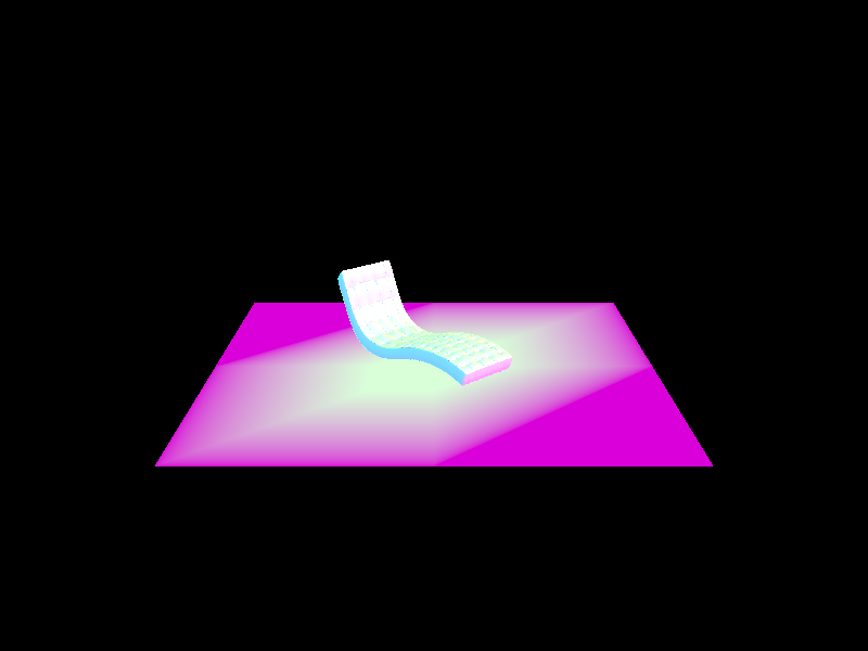
Figure 5: A bench scene containing 67808 primitives.
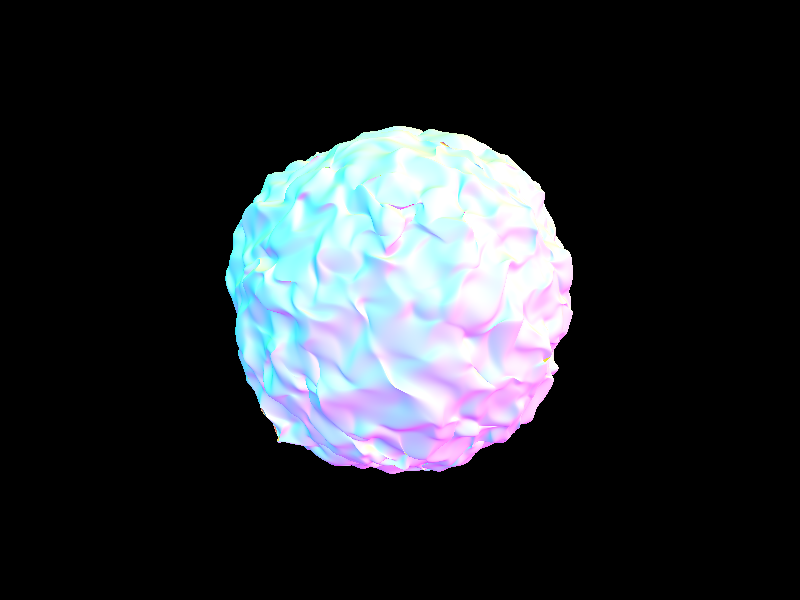
Figure 6: A blob containing 196608 primitives..
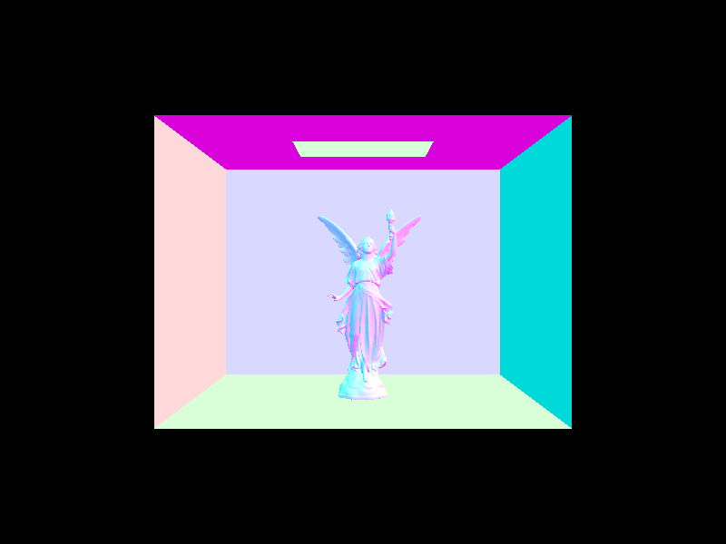
Figure 7: Lucy statue in Cornell box containing 133796 primitives.
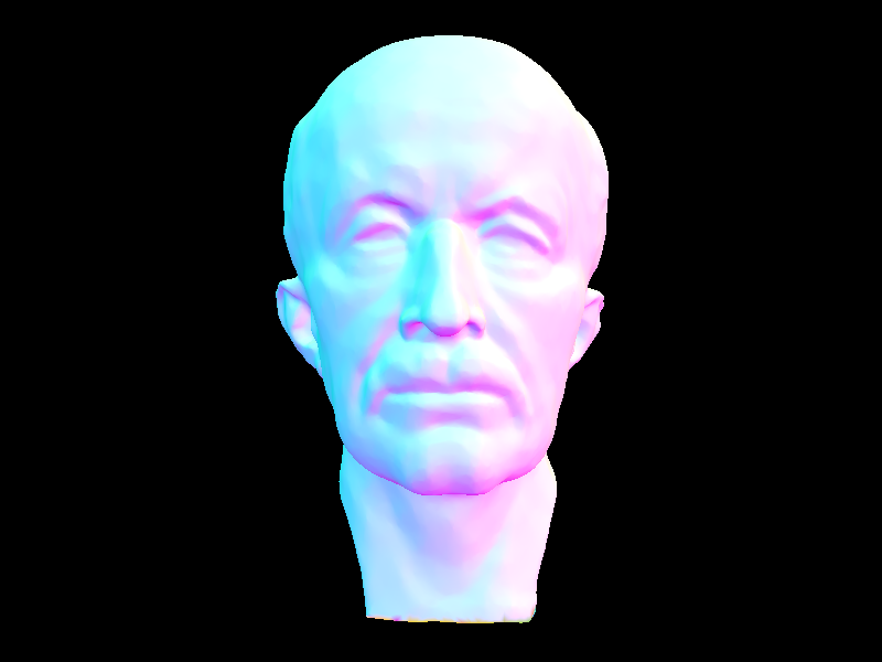
Figure 8: Head of Max Planck containing 50801 primitives.

Figure 9: Scene of Pixar's Wall-E containing 240326 primitives.
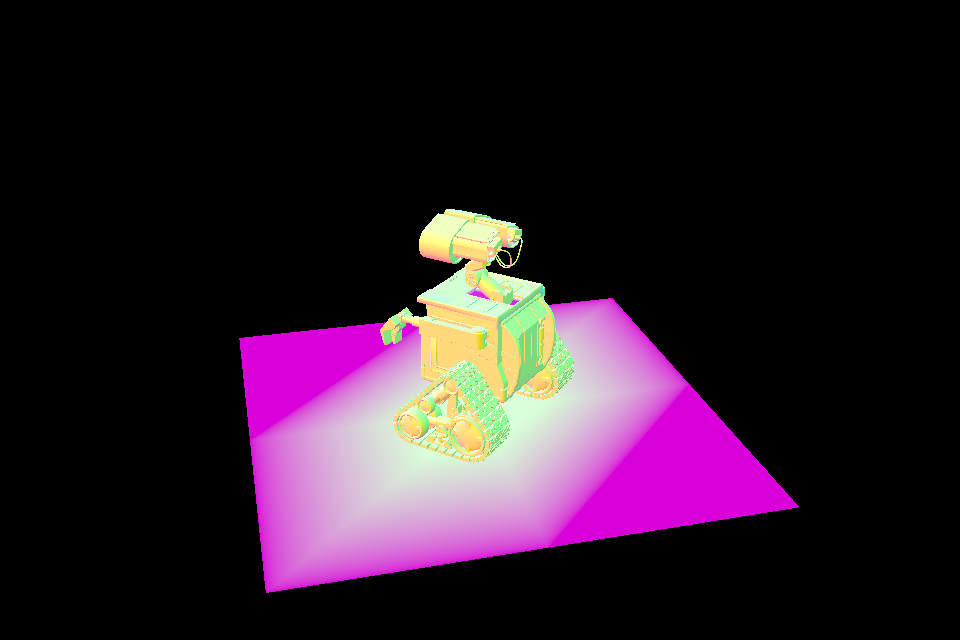
Figure 10: Secondary view of Pixar's Wall-E.
Part 3: Direct Illumination
When implementing the direct lighting function, estimate_direct_lighting() in pathtracer.cpp, the function first creates two matrices, one that transform a vector from object space to world space, o2w, and one that does the opposite, w2o. The point a given ray, r, hits a point at Intersection, isect, is hit_p and is found where
hit_p = r.origin + r.direction * isect.tThe outgoing radiance direction towards the camera in object space, w_out, is given by
w_out = w2o * -r.d;For each light in a given scene, there is a check to see if a light is a delta light. If it is, only one sample is needed to be added to the outgoing radiance, L_out. Otherwise, ns_area_light samples of outgoing radiance are needed per light for a given ray and the average will be added to L_out. To get the outgoing radiance of a sample, hit_p is inputted as an argument for the current light's function sample_L(). This function returns the radiance coming from the light onto hit_p, L_in, direction of the incoming radiance in world space, the distance between hit_p and the light, and the probability that a ray can reach the camera from a ray that hits goes from the light to hit_p, pdf. The incoming radiance direction in world space is converted to the direction of the incoming radiance in object space, w_in. If the cos_theta of w_in compared to the normal vector (0, 0, 1) is positive and the ray from the light towards hit_p doesn't hit anything as it travels to hit_p, the radiance that goes out to the camera, radiance_out, is
radiance_out = L_in * isect->bsdf->f() * cos(wi's theta) / pdfisect->bsdf(bidirectional scatterring distribution function) determines how much radiance goes towards the camera from hit_p due to the material of the surface hit_p is at. After getting ns_area_light samples of radiance_out, we add all the radiance_outs and average the sum.
L_out += sum(radiance_outs) / ns_area_lightL_out is the sum of all the radiance going towards w_out that is calculated from different light sources. Because the radiance is linear, all outgoing radiance can be added together. The Figure 11 to Figure 18 show some bugs faced along the way and final results as well.
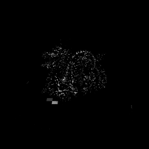
Figure 11: Dragon when Triangle's intersect from part 1 wasn't completely working.

Figure 12: Dragon with no shadows.
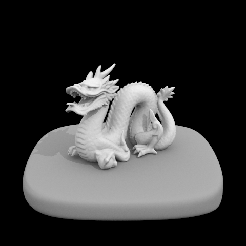
Figure 13: Fixed Dragon with direct lighting.

Figure 14: Building mesh with direct lighting.
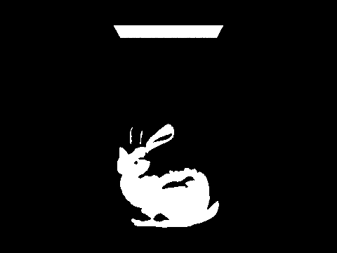
Figure 15: Bunny in Cornell box with conditions to cast shadow mixed up.
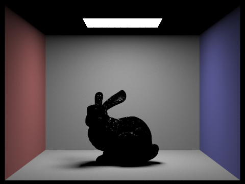
Figure 16: Bunny before Triangle's intersect function from part 1 was fixed.
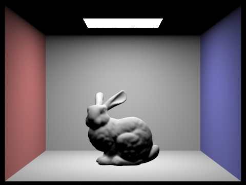
Figure 17: Bunny with no condition to cast shadows.

Figure 18: Fixed Bunny in Cornell Box.
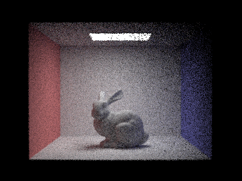
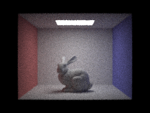
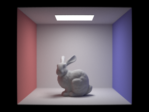
This section focuses on one particular scene to show the change in noise with varying amount of camera rays per pixel. Figure 19 to Figure 26 show 1, 2, 4, 8, 16, 32, 64, and 128 rays per pixel. These figures show that less noise appears as there are more rays per pixel. The input into the terminal that is used was
 ./pathtracer -t 8 -s X -l 32 -m 6 -r 480 360 dae/sky/CBbunny.dae
X = camera rays per pixel(must be power of 2)
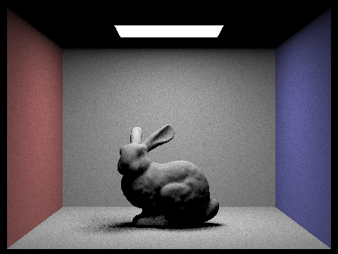
Figure 19: Bunny in Cornell box with 1 camera ray per pixel.

Figure 20: Bunny in Cornell box with 2 camera rays per pixel.

Figure 21: Bunny in Cornell box with 4 camera rays per pixel.
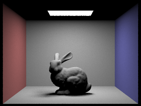
Figure 22: Bunny in Cornell box with 8 camera rays per pixel.

Figure 23: Bunny in Cornell box with 16 camera rays per pixel.

Figure 24: Bunny in Cornell box with 32 camera rays per pixel.

Figure 25: Bunny in Cornell box with 64 camera rays per pixel.

Figure 26: Bunny in Cornell box with 128 camera rays per pixel.
It is easy to see the difference between Figure 19 and Figure 26, 1 versus 128 camera rays per pixel. As the number of rays increase, the picture begins to have less black speckles spread out throughout the image. The soft shadows start as a scattered amount of black pixels that become smooth soft shadows that noticeably lighten at the points that have a lower chance of intersecting the bunny.
Part 4: Indirect Illumination
Next, besides direct lighting from a light source, light bouncing around a scene that find its way to the camera has to be accounted for as well. The light not directly from the light source creates indirect illumination. With both direct and indirect illumination, global illumination is obtained. To calculate this indirect lighting that reaches a pixel using estimate_indirect_lighting() in pathtracer.cpp, the function begins the same as the direct lighting function by getting the point the input ray, r, hits a point in the scene, hit_p, and the outgoing radiance in object space, w_out. We can find the bsdf using isect.bsdf->sample_f(). This function not only calculates the bsdf onto hit_p, but finds the direction the incoming radiance comes from in object space, w_in, and the probability that the incoming radiance will bounce from hit_p and follow w_out. The probability to calculate that this indirect light will bounce to w_out is calculated, prob_term. If the probability is low, the light will probably terminate. Otherwise, w_in is changed to world space from object space, wi, a new ray is created that goes from hit_p to the new wi. Then the incoming radiance is calculated using the function trace_ray(), L_in. The outgoing radiance that hits the pixel using the inputted ray, L_out, is
L_out = L_in * bsdf * cos(w_in's theta) / (pdf * prob_term)L_out is added to all the radiance already calculated from the direct light function to create all the light hitting that point in the scene. Figure 27 to Figure 30 show global illumination. Figure 26 from the last part is the bunny with only direct lighting, but in Figure 27, you can see the shadows become much lighter because rays can reach those areas through indirect lighting. The dragon in Figure 28 is much brighter than the dragon in Figure 13 due to having more light able to hit areas of the dragon. Figure 31 shows Labmertian spheres in a Cornell box with only direct illumination while Figure 32 is that same scene with only indirect illumination. If you add the lighting from the two scenes together, you get Figure 30, the Lambertian spheres in a Cornell box with global illumination.

Figure 27: Bunny with global illumination.

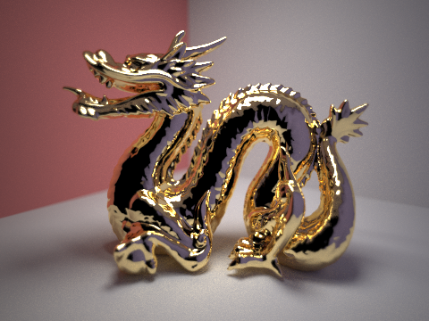
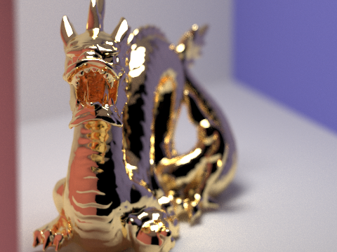
Figure 28: Dragon with global illumination.
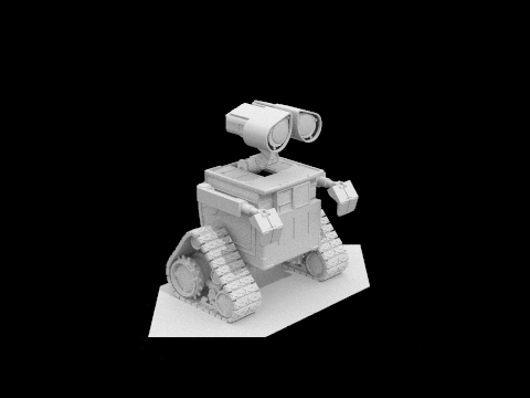
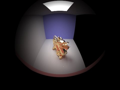
Figure 29: Pixar's Wall-E with global illumination.

Figure 30: Lambertian spheres with global illumination.
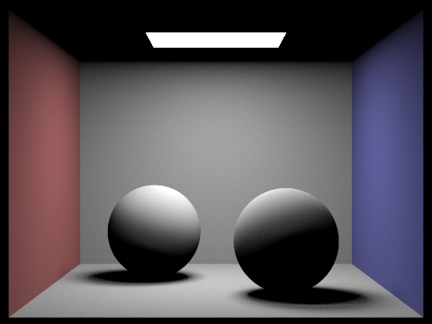
Figure 31: Lambertian spheres with only direct illumination.

Figure 32: Lambertian spheres with only indirect illumination.
This section focuses on one particular scene to show the change in noise with varying values for max_ray_depth. Figure 33 to Figure 40 show 1, 2, 3, 4, 5, 15, 30, and 100 as the values for max_ray_depth. The higher the value for max_ray_depth, the more bounces the rays in indirect illumination have. The input in the terminal was
 ./pathtracer -t 8 -s 64 -l 32 -m X -r 480 360 dae/sky/CBdragon.dae
X = max_ray_depth

Figure 33: Dragon in a Cornell box with max_ray_depth = 1.

Figure 34: Dragon in a Cornell box with max_ray_depth = 2.
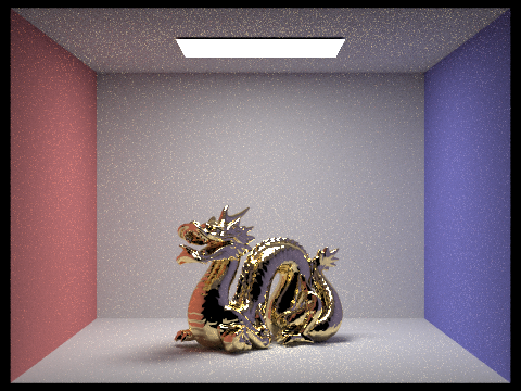
Figure 35: Dragon in a Cornell box with max_ray_depth = 3.

Figure 36: Dragon in a Cornell box with max_ray_depth = 4.

Figure 37: Dragon in a Cornell box with max_ray_depth = 5.

Figure 38: Dragon in a Cornell box with max_ray_depth = 6.

Figure 39: Dragon in a Cornell box with max_ray_depth = 50.
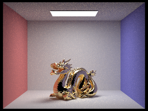
Figure 40: Dragon in a Cornell boxwith max_ray_depth = 100.
The results show that the scene gets noticeably brighter from a max_ray_depth of 1 to 6, Figure 33 to Figure 38, but there is more noise. However, the max_ray_depth of 50 and 100, Figure 39 and Figure 40, both look very similar to the max_ray_depth of 6, Figure 38. There is a little more brightness such as in the mouth of the dragon, but it is still very small amount of change. The small amount of change is because the rays for indirect lighting are less likely to exist as the ray bounces more and more. So the possibility that a ray will bounce 50 or 100 times is really small. The ray will most probably cease to exist by that point.
Using a scene of lambertian spheres in a Cornell box, Figure 41 to Figure 48, like with direct lighting and the bunny in Figure 19 to Figure 26, there is a difference a large difference in the scenes when increasing the sample-per-pixel rate. In this case, 1, 2, 4, 8, 16, 64, 256, and 1024 camera rays per pixel are being used with input into the terminal as
 ./pathtracer -t 8 -s X -l 32 -m 6 -r 480 360 dae/sky/CBspheres_lambertian.dae
X = camera rays per pixel(must be power of 2)
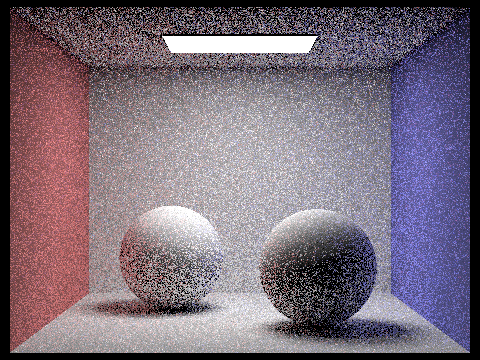
Figure 41: Lambertian spheres in a Cornell box with 1 samples per pixel.
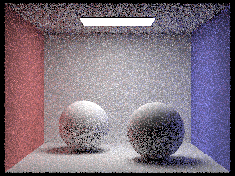
Figure 42: Lambertian spheres in a Cornell box with 2 samples per pixel.

Figure 43: Lambertian spheres in a Cornell box with 4 samples per pixel.

Figure 44: Lambertian spheres in a Cornell box with 8 samples per pixel.
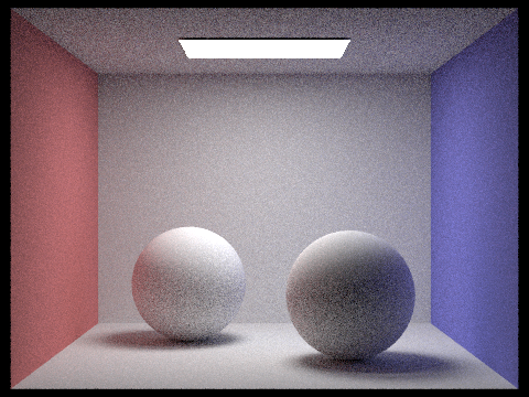
Figure 45: Lambertian spheres in a Cornell box with 16 samples per pixel.

Figure 46: Lambertian spheres in a Cornell box with 64 samples per pixel.

Figure 47: Lambertian spheres in a Cornell box with 2 samples per pixel 256.
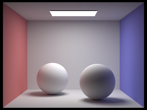
Figure 48: Lambertian spheres in a Cornell box with 1024 samples per pixel.
Unlike just the direct lighting, the noise contribution also comes from the indirect lighting creating white speckles on the rendered image as easily seen in Figure 41 to Figure 45. However, with the increasing samples per pixel rate, the noise starts disappearing as seen in Figure 48 which has 1024 samples per pixel.
Part 5: Materials
Mirror and glass surfaces were implemented as already seen in the Dragon in a Cornell box in the Figure 33 to Figure 40 in Part 4. The materials were implemented by giving mirrors and glass bsdf functions in bsdf.cpp. For a mirror, given vector from the camera onto a hit point, wo, the mirror reflection vector, wi, is first calculated using the normal vector (0, 0, 1).
wi = 2 * dot(n, wo) * n - wo;Since the normal is (0, 0, 1), wi is essentially (-wo.x, -wo.y, wo.z) when using the equation above. However, if the normal vector would be changed, this specific equation would be more important. The mirror bsdf then returns a Spectrum of the mirror's reflectance, given as a parameter for MirrorBSDF objects, divided by the absolute value of the cosine value of new ray, wi, with respect to the normal vector. This bsdf function applies to indirect lights. This function returns the reflectance divided by thr absolute cosine value because it should cancel out the absolute cosine value in pathtracer.cpp's estimate_indirect_lighting() function that was implemented in part 4 of the project. The cosine value needs to be cancelled out because the angle a light hits a point doesn't affect the amount of light leaving a point of a mirror's surface. It just depends on a mirror's ability to reflect light. For direct lights, no light is returned cause direct light can't reflect since it is just 1 ray. Figure 49 shows a mirror sphere in a Cornell box before the glass sphere was implemented.
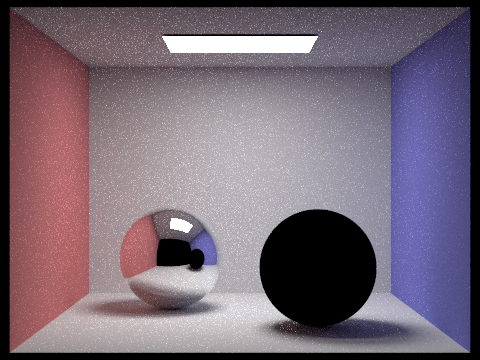
Figure 49: A Cornell box with spheres after mirror surfaces were implemented, but glass surfaces weren't implemented
Glass surfaces were much harder to implement because light rays that pass through a glass object are slightly reflected off the surface while others are refracted. Rays that are refracted enter an object at one angle, go through the object different angle, this angle changes depending on the material of an object, then leaves the object at the same angle it initially came in at. To implement this, there is a check to see if a ray is leaving or entering an object. If wo, the outgoing radiance direction, is entering the outside, the index of refraction, no, is 1, otherwise it is ior, a parameter in a bsdf. The inside index of refraction, ni, is the opposite of no. The ray created due to refraction, wi, is calculated by using Snell's Law where
r = no / ni
l = -wo
c = -dot(n, l)
wi = r * l + (r * c - sqrt(1 - r^2 * (1 - c^2))) * n
r is the ratio of the no and ni. l is negative wo because wo initially points to the hit point from wherever its origin is, the negative sign makes the ray, l, point to the origin and its new origin is its old hit point. c is the dot product of l and the normal vector, n, which is (0, 0, -1) if no is ior, (0, 0, 1) otherwise. since the normal vector lies on the z axis, the x and y values for wi are wo's x and y just scaled by r. The z value of wi is wo's z scaled by r plus a term that adjusts for the change in direction due to refraction. However, if
ni * sin_theta(wi) >= nothen the glass material actually doesn't refract light, it reflects it since total internal reflection occurs. If that happens, the glass is treated as a mirror. Otherwise, Schlick's approximation is used where
r0 = (no - ni) / (no + ni)
p = r0 + ((1 - r0) * (1 - abs_cos_theta(wi))^5)
This p value is used to determine if this ray will be reflected off the glass or refract through the glass. This p value is multiplied by a constant, usually 10 or 20 to make sure at high max_ray_depths, the rays can reach it's max number of bounces before termination. If the p value causes a reflection, the glass sphere is treated like the mirror is before, but the pdf used in pathtracer.cpp's estimate_indirect_lighting() is changed to p and the return value is the same as the mirror, but multiplied by pdf. However, if refraction occurs, pdf is changed to (1 - p) and what is returned is the transmittance, a bsdf parameter, multiplied by r^2, where r is the r when using Snell's law / divided by the absolute value of the cosine value of new ray wi with respect to the normal vector. All of this is multiplied by the pdf.
bsdf = pdf * transmittance * r^2 / abs_cos_theta(wi)The reason for the division of the absolute cosine value is the same as the mirror, but the multiplication by the pdf is because the light ray isn't losing any energy, it is just reflecting or refracting through an object so what is returned is multiplied by pdf to cancel out the pdf pathtracer.cpp's estimate_indirect_lighting(). Figure 50 shows the result of implementing mirror and glass materials, it is the finished version of Figure 49

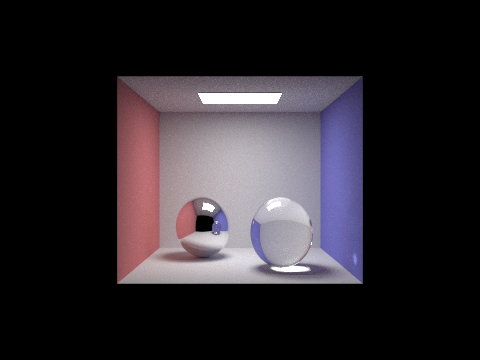
Figure 50: A Cornell box with a mirror sphere and a glass sphere
When rendering the same scene as Figure 50 at muliple max_ray_depth values to see how more bounces of the ray due to an input of the following can affect the renderings.
 ./pathtracer -t 8 -s 1024 -l 32 -m X -r 480 360 dae/sky/CBspheres_.dae
X = max_ray_depth
Figure 51 to Figure 61 show the results of the renderings at different max_ray_depth values.
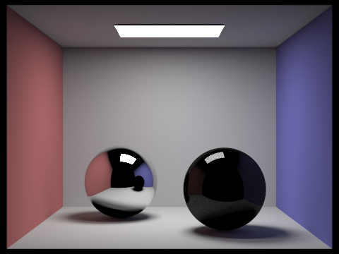
Figure 51: Mirror and glass spheres in a Cornell box with max_ray_depth = 1.
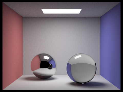
Figure 52: Mirror and glass spheres in a Cornell box with max_ray_depth = 2.
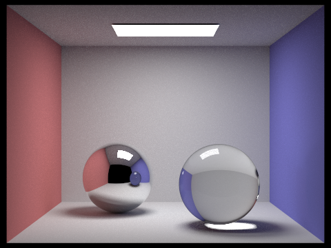
Figure 53: Mirror and glass spheres in a Cornell box with max_ray_depth = 3.
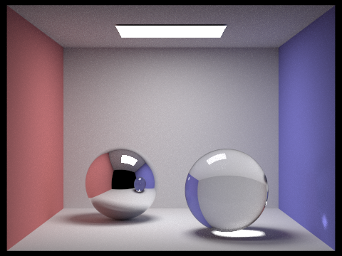
Figure 54: Mirror and glass spheres in a Cornell box with max_ray_depth = 4.

Figure 55: Mirror and glass spheresin a Cornell box with max_ray_depth = 5.
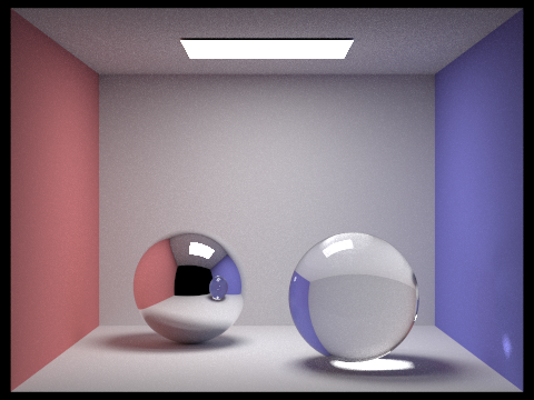
Figure 56: Mirror and glass spheres in a Cornell box with max_ray_depth = 6.

Figure 57: Mirror and glass spheres in a Cornell box with max_ray_depth = 7.

Figure 58: Mirror and glass spheres in a Cornell box with max_ray_depth = 10.

Figure 59: Mirror and glass spheres in a Cornell box with max_ray_depth = 25.

Figure 60: Mirror and glass spheres in a Cornell box with max_ray_depth = 75.

Lastly, since the all the parts of the project are complete, the following shows results with various sample-per-pixel rates, Figure 62 to 69. The various sample rates are 1, 2, 4, 8, 16, 64, 256, and 1024 samples per pixel with arguments into the terminal as
 ./pathtracer -t 8 -s X -l 1 -m 100 -r 480 360 dae/sky/CBspheres.dae
X = camera rays per pixel(must be power of 2)
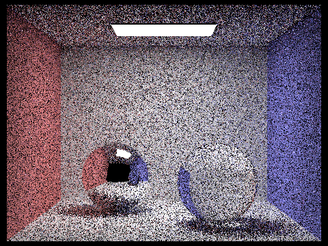
Figure 62: Mirror and glass spheres in a Cornell box with 1 sample per pixel.

Figure 63: Mirror and glass spheres in a Cornell box with 2 samples per pixel.
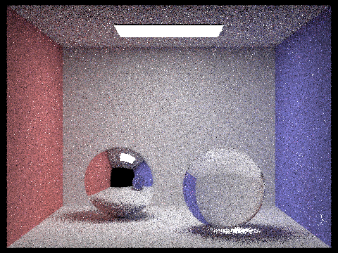
Figure 64: Mirror and glass spheres in a Cornell box with 4 samples per pixel
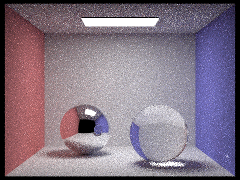
Figure 65: Mirror and glass spheres in a Cornell box with 8 samples per pixel.

Figure 66: Mirror and glass spheres in a Cornell box with 16 samples per pixel.

Figure 67: Mirror and glass spheres in a Cornell box with 64 samples per pixel.
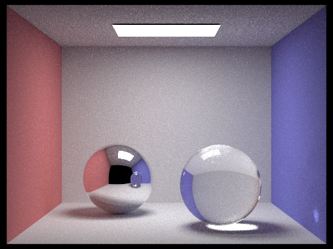
Figure 68: Mirror and glass spheres in a Cornell box with 256 samples per pixel.

Figure 69: Mirror and glass spheres in a Cornell box with 1024 samples per pixel.
As seen in the results of the Figures above more samples per pixel, the less noise. Initially with the first few Figures, there is a lot of white and black noise. However, by 16 samples per pixels, the black noise spots are much less apparent while the white noise is still very noticeable. Yet, by increasing the sample rate all the way to 1024, the result is Figure 69. The noise is barely noticeable and the picture is clear and shows a lot of the detail in shading and lighting.